


Introduction
Community science (CS) datasets have been increasingly utilized to assess a broad range of biological and ecological questions. From 2008 to 2017, approximately 1,700 peer-reviewed publications used CS data (specifically the Global Biodiversity Information Facility; GBIF: https://www.gbif.org/) (); however, by March 2020, that number more than doubled to 4,307 publications (). Many recognize CS data as an extremely valuable source of information for biological research and conservation (; , ; ; ; ; ; ; ), though caution is warranted in relying on these data ().
Community science projects fall along a continuum from unstructured to structured. Structured projects have clearly defined data collection protocols and goals (e.g., Breeding Bird Surveys), whereas unstructured projects lack these characteristics, relying more on opportunistic observations (). Both structured and unstructured projects have advantages and disadvantages. For example, while structured projects may produce more systematic observations, which can reduce sampling bias, the specificity and difficulty inherent in following a collection protocol may reduce the number of participants, thus the amount of data generated. Conversely, unstructured CS projects (frequently conducted using iNaturalist: https://www.inaturalist.org) are more susceptible to spatiotemporal and observer-based biases () but may generate more observations. As of November 2022, iNaturalist had 2.5 million observers who reported more than 135 million species occurrences worldwide (). An important aspect of iNaturalist is a community-based identification process for observations post submission (; ). Observations are classified as “research grade” (RG) when two or more iNaturalist users have agreed on a species-level or finer taxonomic identification. If there is disagreement among identifiers, a greater than two-thirds consensus identification is required for RG status. The majority of scientific research utilizing iNaturalist data includes only RG observations.
Despite the challenges associated with using data generated by unstructured CS projects, iNaturalist has been increasingly used to investigate a broad range of topics, including species distribution modeling (; ; ), phenological studies (), species discovery and rediscovery (; ), and monitoring invasive species (; ; ; ). Thus, a more detailed understanding of the biases associated with iNaturalist data, both for initial recorded observations and the community identification process, is important to ensure accurate conclusions when utilizing this valuable resource.
Spatial biases in data from unstructured CS projects are well documented (; ; ; ; ), including from projects that utilize iNaturalist (). Observation density is often clustered in and around cities and other areas with a high population density (; ). Additionally, certain habitats, land use types, and geographic areas (e.g., terrestrial versus marine, urban greenspaces versus rural areas, and Europe versus Africa) are over- or under-sampled proportionate to their representation in the landscape (; ). Temporal biases are also common in data from CS projects. For example, sampling effort increases on weekends, decreases at night, and decreases during the winter in temperate regions of the Northern Hemisphere (; ; ). In addition to these broad-scale patterns, biases can also occur at the user level, where they are influenced by observer behavior and species’ characteristics.
Understanding bias in the initial reporting of species and the subsequent identification is essential for scientists relying on data from the GBIF because only RG iNaturalist records are part of GBIF. Since unstructured CS projects rely on opportunistic observations submitted by individuals from a wide variety of backgrounds and levels of expertise, user behavior can greatly impact data collection and reporting. Recent studies have shown that iNaturalist observers and identifiers tend to “specialize” in certain taxonomic groups, such as insects, birds, or mammals (; ). Furthermore, even within these broader taxonomic groups, many users focus on certain taxa (e.g., Lepidoptera [butterflies and moths] or Cicindelinae [tiger beetles]). In addition, most iNaturalist observations and identifications are contributed by only a small percentage of users, with the typical iNaturalist observer submitting just a single observation (; ). Among observers that submit more than one observation, many treat iNaturalist as a list-keeping device, submitting only one observation of each species (). Community scientists disproportionately report “conspicuous,” “charismatic,” and “showy” taxa (; ), particularly in unstructured datasets relative to semi-structured (e.g., eBird: https://ebird.org/) (; ). However, the behaviors and morphological features contributing to taxa being showy or conspicuous are not uniform and have not been quantified for most taxonomic groups. Additionally, for iNaturalist datasets, it is equally important to explore how natural history traits influence user interaction during the community identification process, which occurs after submission of observations.
Orbweaving spiders of the family Araneidae are a model taxonomic group in which to explore how natural history traits influence iNaturalist user interactions with different species, from observation through identification. There are many common and widespread orbweaver species that, while varying in size, appearance, and behavior, still share basic natural history traits (e.g., web building, general morphology) that unite them in public perception. Additionally, the recent introduction of a non-native orbweaver into the southeastern U.S. facilitates this exploration of trait-based biases among community scientists within the context of invasive species monitoring. The large-bodied and brightly colored Asian Jorō spider, Trichonephila clavata, was introduced around 2010 to northern Georgia, U.S. (; ). In its introduced range, T. clavata is one of the largest orbweaver species and spins large, golden webs regularly on and around buildings and other artificial structures. This has brought T. clavata to the general public’s awareness, with almost half (3,269/7,019 as of [2023/07/28]) of all iNaturalist observations coming from its smaller, introduced range. These spiders now have an established population in at least four states, spanning an area greater than ~120,000 km2, with additional iNaturalist sightings as far from the center in Georgia as West Virginia and Maryland (; ). Where it has been introduced the longest, T. clavata has become the most common orb weaving spider observed (). Thus, the Jorō spider presents an ideal opportunity to explore further how observers engage with iNaturalist, allowing us to address questions about biases associated with CS data.
We compared how iNaturalist users engaged on iNaturalist with the Jorō spider compared with other common orbweavers across the same geographic area. Some species from other spider families (e.g., Tetragnathidae, Uloboridae) are also known to construct orb webs. We excluded them from this study to restrict our analyses within a single family, Araneidae. Hereafter, we use orbweaver to exclusively describe species in Araneidae. Specifically, we examined which behavioral and morphological traits influenced community scientists when reporting and identifying these species. We expected the more showy species, with bright colors, striking patterns, and large size to drive more community science interaction. We further explored how these traits impacted data quantity and quality, such as the percentage of observations that are RG and the speed with which they achieve that status. Our analysis evaluated both biases in user behavior when reporting species and during the iNaturalist-specific system of community identification. Overall, we analyzed how iNaturalist data quantity and quality is influenced by natural history traits by comparing T. clavata to native orbweavers within its introduced range.
Methods
Dataset
We downloaded all araneid orbweaver iNaturalist observations from the eastern U.S. (east of the Mississippi River) using the iNaturalist API on June 30, 2023. We retained only those observations identified to species level by the iNaturalist community and classified as RG by iNaturalist. RG observations include a photograph, date, coordinates, and a species identity agreed upon by the iNaturalist community. This dataset contained ~118,000 observations by ~47,000 unique users. The oldest observation was from 2009, but 99% were submitted to iNaturalist from 2016 onward. We analyzed observation data for 31 of the most reported species (Supplemental Table 1), all of which had more than 250 RG observations (700+ total).
Assigning behavioral and morphological traits to species
We scored each species in our analysis according to a set of behavioral and morphological traits. We selected traits we hypothesized would influence how iNaturalist users interact with that species rather than a comprehensive treatment of natural history across species. Although we did not use images of male or immature spiders when scoring their characteristics, adult female orbweavers are the most likely to appear in community science observations due to the larger size of their body and web. We chose (1) total body length (mm), (2) presence/absence of bright colors (e.g., colors other than black, gray, or brown), (3) presence/absence of a contrasting color pattern (e.g., stripes, spots), (4) presence/absence of distinctive morphological features (e.g., abdominal spines, leg tufts, hump-shaped abdomens), (5) diurnal presence on web, (6) presence/absence of web stabilimentum or other non-standard web feature (e.g., cultivated web debris), (7) web diameter (cm), and (8) seasonal activity peak. This approach is similar to that of Caley et al. (), and our trait values for each species are displayed in Table 1. Due to a lack of standardized published web-size data for many species, we included body size rather than web size in our final analyses (data for total body length has been published for all species in our analysis). For species where web diameter estimates were available, web size and total body length were highly correlated (r = 0.81).
Table 1
Values of behavioral and morphological traits assigned to study species, with non-native species in bold (World Spider Catalog 2023).
| SPECIES | SIZE (mm) | BRIGHT | CONTRAST | UNIQUE | DIURNAL | SEASON1 | POLYMORPHIC | WEB DECORATION |
|---|---|---|---|---|---|---|---|---|
| Acanthepeira stellata (Walckenaer 1805) | 11.50 | no | no | yes | no | early | no | no |
| Araneus bicentenarius (McCook 1888) | 24.75 | no | yes | yes | no | early | no | no |
| Araneus diadematus2 Clerck 1757 | 13.25 | no | yes | no | yes | late | yes | no |
| Araneus marmoreus Clerck 1757 | 13.50 | yes | yes | no | yes | late | yes | no |
| Araneus nordmanni (Thorell 1870) | 13.00 | no | yes | no | yes | late | no | no |
| Araneus pegnia (Walckenaer 1841) | 5.93 | no | yes | no | yes | late | yes | no |
| Araneus trifolium (Hentz 1847) | 14.50 | yes | yes | no | yes | late | yes | no |
| Araniella displicata (Hentz 1847) | 6.00 | yes | yes | no | yes | early | yes | no |
| Argiope argentata (Fabricius 1775) | 14.00 | yes | yes | yes | yes | early | no | yes |
| Argiope aurantia Lucas 1833 | 23.75 | yes | yes | no | yes | late | no | yes |
| Argiope trifasciata (Forsskål 1775) | 20.00 | yes | yes | no | yes | late | no | yes |
| Cyclosa turbinata (Walckenaer 1841) | 4.25 | no | no | yes | yes | late | no | yes |
| Eriophora ravilla (C. L. Koch 1844) | 18.00 | yes | yes | no | no | early | yes | no |
| Eustala anastera (Walckenaer 1841) | 7.15 | no | no | no | no | early | no | no |
| Gasteracantha cancriformis (Linnaeus 1758) | 8.13 | yes | yes | yes | yes | late | no | yes |
| Gea heptagon (Hentz 1850) | 5.15 | no | no | yes | yes | early | no | no |
| Larinioides cornutus (Clerck 1757) | 10.25 | no | no | no | no | early | no | no |
| Larinioides sclopetarius (Clerck 1757) | 11.00 | no | no | no | no | early | no | no |
| Mangora gibberosa (Hentz 1847) | 9.10 | yes | yes | no | yes | late | no | no |
| Mangora placida (Hentz 1847) | 3.45 | yes | yes | no | yes | early | no | no |
| Mecynogea lemniscata (Walckenaer 1841) | 7.50 | yes | yes | no | yes | early | no | yes |
| Metepeira labyrinthea (Hentz 1847) | 5.85 | no | no | no | no | late | no | yes |
| Micrathena gracilis (Walckenaer 1805) | 8.88 | yes | yes | yes | yes | late | no | no |
| Micrathena mitrata (Hentz 1850) | 6.18 | yes | yes | yes | yes | late | no | no |
| Micrathena sagittata (Walckenaer, 1841) | 7.75 | yes | yes | yes | yes | late | no | no |
| Neoscona arabesca (Walckenaer, 1841) | 7.48 | yes | no | no | no | early | no | no |
| Neoscona crucifera (Lucas 1838) | 14.30 | yes | no | no | no | late | no | no |
| Neoscona domiciliorum (Hentz 1847) | 11.60 | no | yes | no | no | late | yes | no |
| Trichonephila clavata (L. Koch 1878) | 22.38 | yes | yes | no | yes | late | no | no |
| Trichonephila clavipes (Linnaeus 1767) | 28.25 | yes | yes | yes | yes | late | no | no |
| Verrucosa arenata (Walckenaer 1841) | 7.83 | yes | yes | yes | yes | late | no | no |
1 Early/Late = majority of iNaturalist observations submitted before or after August 1, respectively.
2 Bold text indicates species that are introduced to North America (NA). A. diadematus and L. sclopetarius have been present in NA for over a century. The status of G. heptagon is less certain, but it has also been present in NA for an extended period of time.
All authors independently scored brightness, contrast, and presence/absence of distinct morphology for all species using photos of females submitted to iNaturalist within the study area. Traits not scored unanimously were discussed by the authors until a consensus was reached, as in the methodology in . We scored traits for each species based on the appearance and behavior of mature females because these constitute an overwhelming majority of araneid observations on iNaturalist (personal obs.; JFD, AC). We gathered information for other traits from published resources (; ). We report total body length (Table 1) as the mean of the values reported by sources.
During the trait-scoring process described above, we determined that several species (n = 7) exhibit substantial variation in body coloration and patterning (Table 1). For example, Araneus diadematus individuals vary from dull brown to bright orange. We scored these species as “brightly colored” and “contrastingly patterned,” even if certain individuals were not brightly colored or contrastingly marked, and classified them as polymorphic. We ran analyses with and without polymorphic species included. Results did not differ significantly when polymorphic species were excluded, so we present results from the analysis including all species.
Measuring report frequency
To account for different range sizes (as represented on iNaturalist) across species, report frequency was scaled to the number of RG observations per 1,609 km2 (1,000 mi2) of the reported range. We calculated distribution estimates with kernel density estimation (KDE) using the amt R package (). To reduce biases from large-scale spatial patterns, we first filtered observation data to allow only one observation per 20 km2 grid using the spThin R package (). We ran the KDE at 90% coverage to estimate the core reported range of each species.
Quantifying overall user engagement
We calculated a user engagement score (UES) for each user in our dataset as the mean of their number of observations, species reported, and identifications posted on observations from other users. Because of different orders of magnitude in the raw values, these three variables were scaled to µ = 0, sd = 1 before calculating the UES metric. While the UES metric does not perfectly represent the real-world knowledge and experience of each user, it quantifies their engagement with the iNaturalist platform in a single numerical value. Additionally, we believe that in many cases, this metric is an acceptable proxy for experience level among users.
User engagement for each species
In addition to report frequency, we calculated the following values for each species in our analysis: (1) single species observer percentage (% of users having reported at least one observation of that species who have not reported any other species to iNaturalist), (2) percentage of RG observations contributed by single species observers, (3) mean UES of users having reported that species, (4) mean number of times a user reports that species (for casual [<50 observations] and committed [50+] users), (5) mean number of identifications contributed by users on an observation of that species, (6) median time (hours) until an observation of that species is identified by an iNaturalist user (not the original observer), and (7) percentage of observations of that species that are classified as RG.
Modeling how traits influence iNaturalist users
We first used a linear modeling approach to test our hypothesis that behavioral and morphological traits influence the representation of species in the iNaturalist dataset. We also constructed random forest regression models as an alternative method to independently corroborate our linear regression results (). We fitted models for the following four variables: (1) report frequency (normalized by range size), (2) mean UES, (3) number of identifications per observation, and (4) % RG observations. We used these four response variables to analyze observation and identification patterns within the iNaturalist dataset.
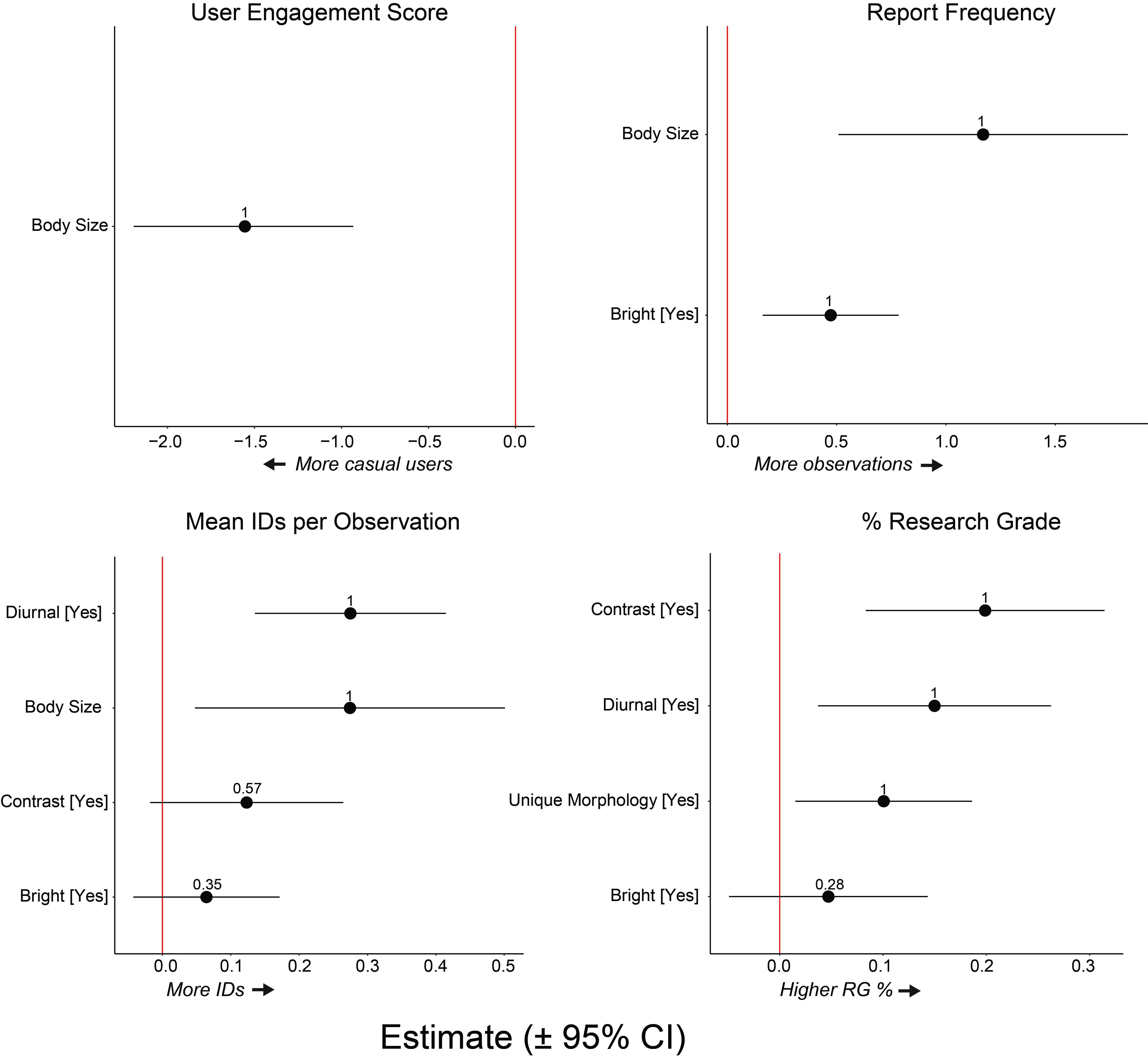
For the linear regressions, we constructed a candidate set of models for each response variable. We performed one-way ANOVAs on each trait for each response variable. Traits with a significant or near-significant effect (p < 0.10) were included in the “global” model for that response variable. We examined the homogeneity of residuals by plotting model residuals against model-fitted values. We visually inspected quantile-quantile plots to confirm model residuals were normally distributed. We performed model selection based on second order Akaike’s Information Criterion (AICc) adjusted for small sample sizes, using the MuMIn R package () and ranked candidate models by ΔAICc (). We averaged statistically indistinguishable candidate models (ΔAICc < 2) to obtain coefficient estimates for fixed effects. If one model performed significantly better than all other models (ΔAICc > 2), we reported coefficient estimates for that candidate model. We summed Akaike weights (wi) across all candidate models to evaluate the relative importance of each fixed effect. If a parameter had a 95% confidence interval not overlapping zero, we concluded that the parameter had a significant effect on the response variable. The linear regression analyses were conducted in R v. 4.1.1.
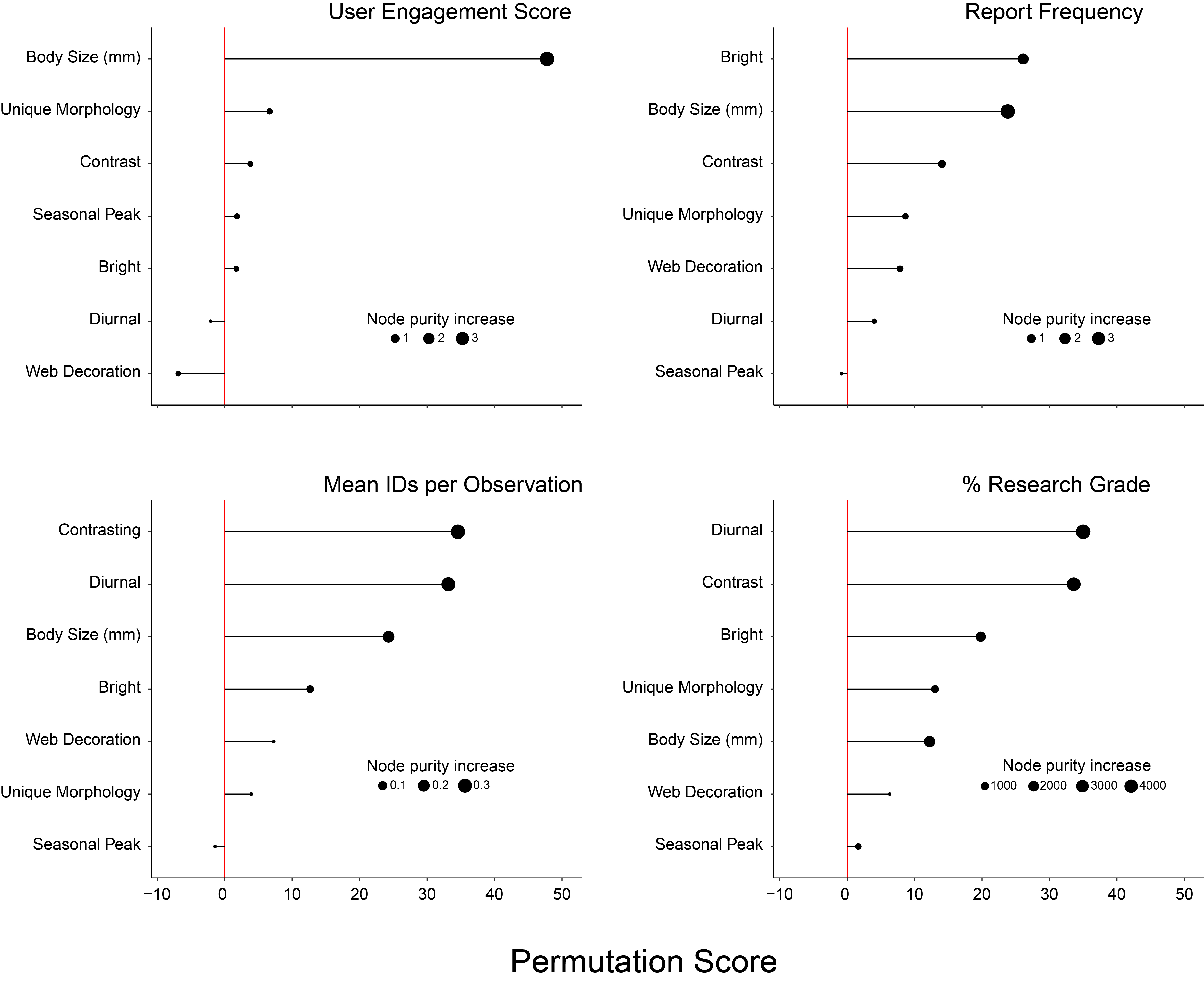
The random forest algorithm is a machine-learning technique that combines the results of many individual, independent trees into a consensus tree. It uses a bootstrap aggregation approach that samples a subset of the data with replacements for each tree constructed. It then combines all the trees using majority vote or averaging, depending on whether the algorithm is used for classification or regression. Because a random forest methodology may perform better than AIC for large datasets (), we also used the randomForest package (version 4.7–1.1; ) to construct regression models for each response variable, including all predictor variables except web size (see above). We used a gridded search to tune our hyperparameters, that is, parameters that must be specified before running each model, in this case, mytr (the number of variables randomly sampled at each split), sampsize (size of sample data drawn at each node), and nodesize (minimum size of terminal nodes). We selected the values for each hyperparameter that minimized the out-of-bag (OOB) error rate and ran 2,000 trees per model. We used both the randomForest and randomForestExplainer (version 0.10.1; ) packages to evaluate model coverage and variable importance. We evaluated model performance by splitting our data into 5 folds and calculating the R2 between actual and estimated dependent variables. We did this five times for each dependent variable using a different fold for testing each time and report the average R2. All data analyses were performed in R v. 4.3.1 ().
Results
Influence of natural history traits
Overall, the linear regression and random forest results were very similar. We observed only a few cases where the random forest analysis supported an additional variable not identified by the linear regression. However, both methods consistently identified similar variables as predictive of reporting and engagement metrics.
The top-performing linear regression model for mean UES was statistically distinguishable (ΔAICc > 2) and accounted for 75% of the total model weight. The top-performing model accounted for 45% of the variance in mean UES. Body size (LM: z = 5.07, p < 0.001) was a significant predictor of mean UES for a species. The random forest model (average R2 = 0.85) predicted 31% of the variance in mean UES and body size was the most important predictor of mean UES (Table 2).
Table 2
Modeling results. Traits are shown in the table if they were included in the top-performing Linear Regression models or with >10% increase in mean squared error (MSE) in the Random Forest model. ID: identification, RG: research grade, UES: user engagement score.
| RESPONSE | LINEAR REGRESSION | RANDOM FOREST | |||||
|---|---|---|---|---|---|---|---|
| PARAMETER | ESTIMATE | CI | WEIGHT | % INCREASE MSE | INCREASE NODE PURITY | EFFECT | |
| User engagement | |||||||
| Size | –1.56 | –2.19, –0.93 | 1.0 | 47.79 | 3.85 | UES decreases with size. | |
| Report frequency | |||||||
| Bright | 0.47 | 0.16, 0.78 | 1.0 | 26.12 | 1.87 | Bright colors increase reports. | |
| Size | 1.17 | 0.51, 1.83 | 1.0 | 23.81 | 3.58 | Reports increase with size. | |
| Contrast | – | – | – | 14.07 | 0.86 | Contrast increases report. | |
| IDs per observation | |||||||
| Contrast | 0.12 | –0.02, 0.26 | 0.57 | 34.57 | 0.32 | Contrast increases IDs. | |
| Size | 0.27 | 0.05, 0.50 | 1.0 | 24.29 | 0.19 | IDs increase with size. | |
| Diurnal | 0.28 | 0.14, 0.41 | 1.0 | 33.16 | 0.30 | Diurnal activity increases IDs. | |
| Bright | – | – | – | 12.66 | 0.06 | Bright colors increase IDs. | |
| RG % | |||||||
| Contrast | 0.20 | 0.08, 0.31 | 1.0 | 33.6 | 3763 | Contrast increases RG %. | |
| Diurnal | 0.15 | 0.04, 0.26 | 1.0 | 35.0 | 4251 | Diurnal activity increases RG %. | |
| Unique | 0.10 | 0.02, 0.19 | 1.0 | 13.04 | 865 | Unique morphology increases RG%. | |
| Bright | – | – | – | 19.8 | 1785 | Bright colors increase RG % | |
The top-performing linear regression model for report frequency was statistically distinguishable (ΔAICc > 2) and accounted for 75% of the total model weight. The top-performing model accounted for 46% of the variance in report frequency. Body size (LM: z = 3.62, p = 0.001) and the presence of bright colors (LM: z = 3.12, p = 0.004) were significant predictors of report frequency. The random forest model (average R2 = 0.97) predicted 35% of the variance in report frequency. Body size and the presence of bright colors were the most important (i.e., had the greatest permutation scores) predictors of report frequency (Table 2).
The four top-performing linear regression models for mean identifications per observation were statistically indistinguishable (ΔAICc < 2) and accounted for 68% of the total model weight (Supplemental Table 2). The top-performing model accounted for 68% of the variance in mean identifications per observation. Body size (LM: z = 2.28, p = 0.03) and diurnal presence on the web (LM: z = 3.94, p < 0.001) were significant predictors of identifications per observation (Supplemental Figure 1). The random forest model predicted 67% of the variance in identifications per observation. The random forest model (average R2 = 0.98) also found that body size and diurnal presence on the web were important predictors of identifications per observation. However, the random forest model also found that the presence of contrasting color patterns had a greater permutation score than body size (Table 2; Supplemental Figure 2).
The two top-performing linear regression models for % RG were statistically indistinguishable (ΔAICc < 2) and accounted for 61% of the total model weight. The top-performing model accounted for 69% of the variance in % RG. The presence of contrasting color patterns (LM: z = 3.73, p < 0.001), diurnal presence on the web (LM: z = 2.80, p = 0.01), and presence of distinct morphological features (LM: z = 2.41, p = 0.02) were significant predictors of % RG (Figure 1). The random forest model (average R2 = 0.97) predicted 66% of the variance in % RG. Similar to the linear regression results, diurnal presence on the web, the presence of contrasting color patterns, and the presence of distinct morphological traits were the most important predictors of % RG. However, the random forest models found that the presence of bright colors had a greater permutation score than the presence of unique morphological traits (Table 2).
Influence of morphological traits on the percentage of iNaturalist observations for a species that are classified as research grade.
Representation in iNaturalist dataset
After accounting for variation in geographic distribution, the most frequently reported species were T. clavata, as well as Argiope argentata, Trichonephila clavipes, Gasteracantha cancriformis, and Argiope aurantia. The least frequently reported species were Eustala anastera, Acanthepeira stellata, Mangora gibberosa, Metepeira labyrinthea, and Larinioides sclopetarius (Supplemental Table 1).
Few (3.1%) iNaturalist users in the dataset reported only a single species to iNaturalist. Among species included in our analysis, T. clavata was reported the most frequently by single-species users, with 10.8% of T. clavata observers reporting only this species (Figure 2). The species with the second highest report rate from single-species users was Eriophora ravilla (3.2%), and over half of the species were reported by less than 1% of such users. Six species had no single-species user observations, including Cyclosa turbinata and Neoscona arabesca. Only 1.3% of observations in the dataset were contributed by single-species users, and of these, T. clavata had the highest percentage of reports (7.6%) contributed by such users. The next highest report rates were from E. ravilla and A. diadematus with 2.3% each. Twenty-two species in our dataset had less than 1% (Supplemental Table 1).
Percentage of iNaturalist observations reported by single-species users plotted against percentage of single-species users for each species included in analysis.
The mean user engagement score (UES) for a species strongly correlated with the range-corrected report frequency of that species in the dataset (Figure 3). Species reported more frequently were reported by less-engaged users (lower mean UES), and species reported less frequently were reported more often by more-engaged users (higher mean UES). Overall, UES decreased with size, with T. clavata having the lowest UES among the species included in the analysis (Supplemental Table 1), followed by A. aurantia, Araneus marmoreus, Neoscona crucifera, and A. diadematus.
Mean user engagement score (UES) among users reporting a species plotted against the number of research grade (RG) observations of that species per 1000 miles2 of range. Lower UES scores indicate species typically reported by more casual iNaturalist users, whereas higher scores indicate species typically reported by more committed iNaturalist users. The dotted line represents the average engagement level of users among analyzed species. Species represented with photos are marked with an asterisk.
Species with bright colors, larger size, and more visual contrast were reported more often (Table 2). Most users reported only 1 observation per species, and 80% of species-observer pairs in the dataset were represented by a single observation. Among both casual (<50 observations) and committed (50+ observations) iNaturalist users, T. clavata and Eustala anastera had the highest and lowest mean number of reports per user, respectively (Figure 4).
Number of observations reported for each species by individual users. Mean and 95% confidence interval is reported for users with more than 50 total observations and for users with less than 50 total observations. These two groups correspond with the top two thirds and bottom third of users by UES, respectively. Species represented with photos are marked with an asterisk.
The mean and median number of identifications (not counting those by the original observer) made on an observation were 1.1 and 1, respectively. Identifications were increased in species with more contrast, larger size or bright colors, or diurnal activity (Table 2). Species with the highest mean number of identifications per observation were T. clavata (2.33), T. clavipes (1.83), G. cancriformis (1.57), and the three Argiope species (Supplemental Table 1). Species with the lowest mean number of identifications per observation were L. sclopetarius (0.30), E. anastera (0.34), and N. crucifera (0.45).
The median time until the first identification by an iNaturalist user was 17.2 hours. Species with the fastest time to identification included T. clavata (1.1 hours), G. cancriformis (1.4 hours), and A. aurantia (1.5 hours) (Supplemental Table 1). Species with the longest time until identification were M. gibberosa (15 days), A. diadematus (2 days), and Mecynogea lemniscata (2 days).
At the time of analysis, most (81%) of the observations of analyzed species were classified as RG (identifications occasionally lose RG status, see ). Overall, species with a higher contrast, diurnal activity, unique morphology, or bright colors tended to contribute to an increased percentage of RG observations (Table 2). Species with the highest percentage of observations classified as RG were G. cancriformis (99.3%), A. aurantia (99.1%), and T. clavipes (99.0%). Species with the lowest percentages were L. sclopetarius (20.8%), E. anastera (23.8%), and N. crucifera (31.2%). Nearly all T. clavata observations (96.1%) were RG (Supplemental Table 1).
Discussion
Analyses of iNaturalist records revealed how the representation of species in a community science dataset is influenced by interactions between species’ traits and observer behavior. Notably, the recently introduced T. clavata is a clear outlier across numerous metrics, having generated widespread reporting and high levels of community engagement compared to a similar congener, T. clavipes, and other orbweavers. This invasive species provides valuable insight into community science, monitoring of new non-native species, and biases in datasets.
Both of our analyses found that orbweaver body size predicted multiple aspects of iNaturalist user behavior, from how frequently species were reported, to the degree of user engagement, and even the number of identifications for each observation. This corroborates findings from studies on insects (), birds (; ), molluscs (; ), and reptiles () that show larger species are reported more often. Spider body size and its correlated trait, web diameter, may be particularly important since it influences the probability of detection in nature. In fact, body size may interact strongly with other morphological traits we considered; for instance, bright or contrasting color patterns may be more easily perceived on larger species than on smaller species.
Body size also influences the difficulty of taking a clear photograph of a subject (; ; ). This may be especially true for casual users taking photos with a smartphone, which may not have the macrophotography capabilities to capture crisp images of small subjects. Blurry photos may then deter users from uploading to iNaturalist or reduce the willingness of other users to engage, as low image quality makes it difficult to distinguish features necessary to identify subjects to species ().
Both analyses revealed that physical and behavioral traits influenced community science engagement, where bright and contrasting coloration, unique and larger body morphologies, and diurnal activity predicted multiple metrics of user engagement. Distinctive coloration, notable appearance, and larger body size are all known to contribute to the visual charisma of species (; , ; ). A striking appearance, along with the perceived noteworthiness or novelty of a species, likely boosts iNaturalist user engagement (; ). This creates a bias in the data available to researchers through GBIF, as only RG observations are included. Distribution maps of less striking species should be viewed skeptically when generated from community science sources ().
Our case study, T. clavata, is large, diurnally active, and has bright contrasting color patterns. Additionally, it received a barrage of sensationalist media coverage in 2022 as a recent invader (), with media outlets speculating that “[z]illions of large Jorō spiders could invade [the] U.S. East Coast” and calling for community members to watch out for their impending arrival. Potentially in response, multiple projects were launched on iNaturalist, dedicated to encouraging users to upload observations with the goal of tracking this species. Heightened public awareness of “giant parachuting spiders coming [their] way” in addition to this species possessing a full suite of conspicuous traits has likely created ideal conditions for high user engagement.
We believe these circumstances have allowed T. clavata to become a “gateway species” into iNaturalist, drawing users to the app solely to document the invasion. Indeed, among the species analyzed, T. clavata had the greatest proportion of observations reported by users who have not reported any other species (Figure 2). Users also repeatedly submitted observations of T. clavata, breaking with the more typical species checklist behavior on iNaturalist (Figure 4). This pattern was notable for both casual and committed iNaturalist users, indicating that observers of all experience levels interact with T. clavata in a unique way compared with native orbweavers. This could be reflective of observers being motivated to document the range expansion of this non-native species.
T. clavata also represents an extreme in the dataset by having the most observations from the least experienced users (Figure 3). The accessibility of T. clavata to novice users is likely attributable to its large body size, striking color patterns, and substantial web. Indeed, the four species with the most observations from the least engaged users (T. clavata, T. clavipes, A aurantia, and G. cancriformis) all have some combination of those eye-catching traits. It is notable that the native golden orbweaver, T. clavipes, does not exhibit a pattern of observations as extreme on iNaturalist, considering it has similar web and body features as its close relative, T. clavata (). Although T. clavipes is a larger species, the density of its observations corrected for its range size is under half of that for T. clavata. This sheds light on the likely effect of a well-publicized, invasive species in piquing the interest of community scientists.
Our study shows that species’ traits bias every step of the iNaturalist process, from recording an observation, receiving user identifications, to achieving RG status. These compounding biases can limit the usefulness of community-level datasets to infer relative species abundance, as less striking species will be poorly represented in frequently used data sources such as GBIF. While research on species like T. clavata benefits from the increased engagement of both casual and committed iNaturalist users, data on small, less conspicuous species likely suffer from underreporting, misidentifications, or a lack of identifications. This is particularly true of species that cannot be identified without the help of magnification, dissection, chemical analyses, or sequencing (). Thus, the frequency of observations between species should not be used to infer real-life differences in species’ abundance without acknowledging the role of species’ characteristics in report and identification frequency. While distribution maps made from iNaturalist observations of highly engaging species might be relatively accurate, the opposite is likely true of small, less conspicuous species. These biases are especially important to consider when tracking invasive species, since species lacking striking traits will be less likely to be reported by community scientists ().
Considering the documented biases of community science data sets, we provide the following recommendations to researchers on how to maximize their benefits from using iNaturalist data, especially when studying small species lacking distinct colors or patterns:
- Conduct outreach on species of interest. Researchers can bring awareness to species of interest within iNaturalist by creating projects and journal posts, and by sharing resources in the iNatForum. Advertising a research need to find particular species can provide a sense of purpose, motivating users to contribute observations. Project descriptions should clearly detail the research aims and any additional information and features to be requested, for example, the inclusion of plant hosts and substrates in photographs or details about sex, life stage, or invasive status. Including information about the size of the organism and how to distinguish it from similar species will improve the quality of data collected. Connections with iNaturalist users may also provide the opportunity to collect specimens (e.g., for DNA analyses). Using iNaturalist to make structured projects will be more useful for obscure taxa (), especially if coupled with active recruitment and training (). Recruitment and training can occur during public outreach events, media interviews, and extension workshops. Social media and cross-platform posts can be an effective means of sharing iNaturalist projects and sparking public interest.
- Engage with the community, especially with experienced users. We encourage researchers to view iNaturalist as a community in which to invest and reciprocally contribute, not just a platform from which to extract data. Intermediate and advanced users are particularly worth engaging with by providing feedback on identifications and comments on distinguishing traits of species. By spending time engaging in refining identifications, researchers will increase the quality of community science data by increasing the number of RG observations and challenging any observations incorrectly regarded as RG. Currently, approximately 60% of observations and 75% of identifications are made by the top 1% of users (; ). Advanced users often already possess strong taxonomic skills, specializing on specific groups of interest (), and may even relish the challenge of searching for small, dull, and rare species in the field (). Providing links to useful resources such as reputable regional guides and taxonomic keys as well as updates on an iNaturalist project can also encourage continuous user engagement. We also recommend offering co-authorship or credit in the acknowledgements section of a paper to recognize substantial contributions.
- Upload data from surveys to iNaturalist. Taxonomic biases in iNaturalist datasets may be improved if researchers upload geotagged photographs from structured survey datasets. Data from structured surveys utilizing systematic methods to locate species of interest (e.g., use of UV lights for moths) or conducted outside of typical circumstances (e.g., nocturnally) may help provide a more accurate record of species diversity and distributions. iNaturalist has a computer vision model that uses machine learning approaches to suggest identifications to users. Uploading accurately identified photographs, especially of obscure species, can add new taxa to the model as well as refine its identification capabilities. These photographs can also provide more reference material for the community, especially if certain species are not already known to a region on the app. Amidst concerns of biodiversity declines (; ), media-based collections and CS datasets will play an increasingly important role in future biodiversity and taxonomic research.
Conclusion
Representation of species in community science datasets is influenced by characteristics of species being recorded, patterns of user behavior, and the interactions between these two factors. We used T. clavata as an example to highlight the power of iNaturalist as a community science tool and to explore observation and identification biases in the dataset. Natural history characteristics drive representation in the iNaturalist dataset, but T. clavata indicates that public awareness from media coverage may also play an important role. Researchers using community science datasets to monitor invasive species, or otherwise, should be conscientious of these biases to ensure accurate interpretation of the data provided by iNaturalist and other CS projects. Our recommendations should result in more RG observations, which are of the greatest value to scientific endeavors. Data quality is, in part, a reflection of community scientist engagement, arguing for researchers to be active participants in the broader community.
Data Accessibility Statement
R scripts and raw data used in this study are available via Zenodo at https://doi.org/10.5281/zenodo.10569983.
Supplementary Files
The Supplementary files for this article can be found as follows:
Supplemental Table 1Calculated metrics for study species. Obs: research grade observations, SSO: single-species observers, UES: user engagement score, RG: research grade. DOI: https://doi.org/10.5334/cstp.690.s1
Supplemental Table 2Top-performing candidate models for four response variables. DOI: https://doi.org/10.5334/cstp.690.s2
Supplemental Figure 1Importance of traits for predicting user engagement score (UES), report frequency, identifications per observation, and % research grade. Figure shows CI 95 estimate for parameters included in top-performing models. Number indicates sum of parameter weight. DOI: https://doi.org/10.5334/cstp.690.s3
Supplemental Figure 2Importance of traits for predicting user engagement score (UES), report frequency, identifications per observation, and % research grade. Figure shows % mean squared error (MSE) per parameter. Size of dot indicates node purity increase. DOI: https://doi.org/10.5334/cstp.690.s4